Very often, when studying financial series, their smoothing is used. You can use anti-aliasing to remove high-frequency components –
they are considered to be caused by random factors and are therefore insignificant. Smoothing always involves some method of averaging
data, in which random changes in the time series mutually absorb each other. Most often, the following methods are used for this purpose:
simple or weighted moving average, as well as exponential smoothing.

Each of these methods has its own advantages and disadvantages. So, a simple moving average is simple and clear, but for its application
the relative stability of the periodic and trend components of the time series is required. Also, for the moving average
the signal delay is characteristic. The exponential smoothing method is free from the lag effect. But even here there are flaws –
exponential smoothing is only effective when the series is aligned with random outliers. 

A reasonable trade-off between a simple and exponential average is to use a weighted moving average. However, here it gets up
the problem of choosing specific weight values. Let’s try to understand this issue together.

So, first, let’s define what we would like to achieve from the smoothing procedure:

• first, we need to remove random changes and noise from the price series;

* secondly, we would like to detect abnormal emissions and unusual price behavior, which also
can be used in trading;

* finally, the averaging procedure should identify stable trends if they are
present on the market.

And, of course, we would like the smoothing procedure to adapt to the current market situation.

In order to get the desired result, we will calculate the weight coefficients depending on how far
this price level is located from the maximum and minimum prices for the study period. Thanks to this approach, we will get a filter
that performs the smoothing procedure depending on the price distribution for the period of interest.

The main advantage of this smoothing algorithm is its stability in relation to various types of outliers: price deviations
they may be very large, but the filter will still follow the most significant trends. In addition, with different source data
we can get essentially different effects. So, if the prices are distributed more or less evenly, then we get a filter
the moving median. If the prices accumulate around one value and the difference between the maximum and minimum is large enough, we will get
modal smoothing. If all prices are within a very narrow range, we will get a simple moving average.

The main disadvantage of this method is that the smoothing is performed without taking into account price changes over time. Indeed, we can
however you want to change the order of prices within the analyzed period – this will not affect the result of calculations in any way. So
Thus, we can say that this algorithm considers the price change as a random process.

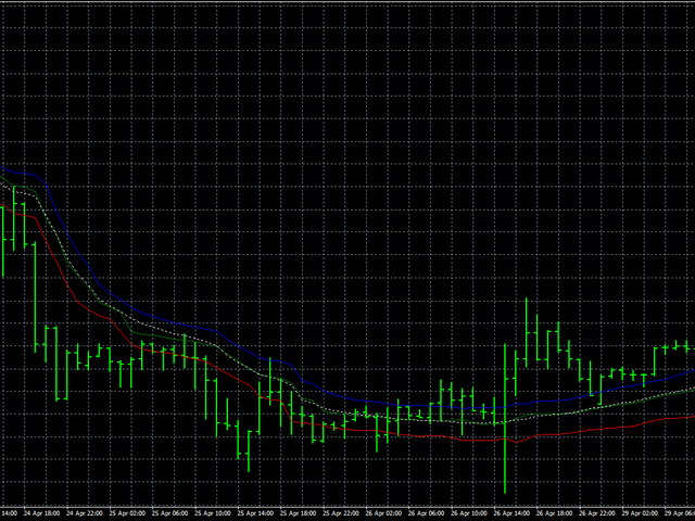
Despite this drawback, let’s see how this algorithm works on real data. In this case, we will proceed as follows: first
we will smooth out the Open, High and Low prices separately from each other, and then all the prices together. Smoothing all prices at the same time will allow us to
to judge how stable the price behavior is in general. The blue line will show the High price smoothing, the red line will show the Low price smoothing, and the green line will show the Low price smoothing.
the line will indicate the smoothing of the opening prices. The white dotted line shows the smoothing of all prices at the same time.

Add review

Reviews ( 0 ):